Notes on Regression - Singular Vector Decomposition

Here's a fun take on the OLS that I picked up from The Elements of Statistical Learning. It applies the Singular Value Decomposition, also known as the method used in principal component analysis, to the regression framework.

Singular Vector Decomposition (SVD)

First, a little background on the SVD. The SVD could be thought of as a generalisation of the eigendecomposition. An eigenvector v of matrix $\mathbf{A}$ is a vector that is mapped to a scaled version of itself:

where $\lambda$ is known as the eigenvalue. For a full rank matrix (this guarantees orthorgonal eigenvectors), we can stack up the eigenvalues and eigenvectors (normalised) to obtain the following equation:

where $\mathbf{Q}$ is an orthonormal matrix.

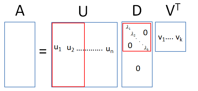
For the SVD decomposition, $\mathbf{A}$ can be any matrix (not square). The trick is to consider the square matrices $\mathbf{A}'\mathbf{A}$ and $\mathbf{A}\mathbf{A}'$. The SVD of the $n \times k$ matrix $\mathbf{A}$ is $\mathbf{U}\mathbf{D}\mathbf{V}'$, where $\mathbf{U}$ is a square matrix of dimension $n$ and $\mathbf{V}$ is a square matrix of dimension $k$. This implies that $\mathbf{A}'\mathbf{A} = \mathbf{V}\mathbf{D}^{2}\mathbf{V}$ and $\mathbf{V}$ can be seen to be the eigenvalue matrix of that square matrix. Similarly, the eigenvectors of $\mathbf{A}\mathbf{A}'$ forms the columns of $\mathbf{U}$ while $\mathbf{D}$ is the square root of the eigenvalues of either matrix.

In practice, there is no need to calculate the full set of eigenvectors for both matrices. Assuming that the rank of $\mathbf{A}$ is k, i.e. it is a long matrix, there is no need to find all n eigenvectors of $\mathbf{A}\mathbf{A}'$ since only the elements of the first k eigenvalues will be multiplied by non-zero elements. Hence, we can restrict $\mathbf{U}$ to be a $n \times k$ matrix and let $\mathbf{D}$ be a $k \times k$ matrix.

Here's a paint illustration of the dimensions of the matrices produced by the SVD decomposition to illustrate the idea more clearly. The $n \times k$ matrix produced by multiplying $\mathbf{U}$ and $\mathbf{D}$ is equivalent for both the blue (keeping all n eigenvectors) and red (keeping only the relevant k eigenvectors) boxes.

Applying the SVD to OLS

To apply the SVD to the OLS formula, we re-write the fitted values, substituting the data input matrix $X$ with its equivalent decomposed matrices:

where the third to fourth line comes from the fact that $(\mathbf{D}'\mathbf{D})^{-1}$ is a $k \times k$ matrix with the square root of the eigenvalues on the diagonal, and $\mathbf{D}$ is a square diagonal matrix. Here we see that the fitted values are computed with respect to the orthonormal basis $\mathbf{U}$.¹

Link to the ridge regression

The ridge regression is an OLS regression with an additional penalty term on the size of the coefficients and is a popular model in the machine learning literature. In other words, the parameters are chosen to minimalise the penalised sum of squares:

The solution to the problem is given by: $\hat{\beta}^{ridge} = (\mathbf{X}'\mathbf{X} + \lambda I_{k})^{-1}\mathbf{X}'\mathbf{Y}$. Substituting the SVD formula into the fitted values of the ridge regression:

where $\mathbf{u}$ is a n-length vector from the columns of $\mathbf{U}$. This formula makes the idea of regularisation really clear. It shrinks the predicted values by the factor $d^{2}_{j}/(d^{2}_{j} + \lambda)$. Moreover, a greater shrinkage factor is applied to the variables which explain a lower fraction of the variance of the data i.e. lower $d_{j}$. This comes from the fact that the eigenvectors associated with a higher eigenvalue explain a greater fraction of the variance of the data (see Principal Component Analysis).

The difference between how regularisation works when one uses the Principal Component Analysis (PCA) method vs the ridge regression also becomes clear with the above formulation. The PCA approach truncates variables that fall below a certain threshold, while the ridge regression applies a weighted shrinkage method.