Thesis Thursday 5 - From recipes to weights

In the previous post, I provided an exploratory analysis of the allrecipe dataset. This post is a continuation and details the construction of product weights from the recipe corpus.

TF-IDF

To obtain a measure of how unique a particular word is to given recipe category, I calculate each word-region score using the TF-IDF approach which is given by the following formula:

TF\text{-}IDF_{t,d} =\frac{f_{t,d}}{\sum_{t'\in d}f_{t',d}} \cdot log \frac{N}{n_{t}+1}

where $f_{t,d}$ is the frequency in which a term, $t$ , appears in document $d$ , $N$ is the total number of documents in the corpus and $n_{t}$ is the total number of documents where term $t$ is found.

The first term takes the number of times a particular word appears in a document and normalise it against the document length. This is also known as the term frequency (TF). The second term takes the logarithm of the ratio of the total number of documents divided by the frequency which the term is found across all documents in the corpus and is known as the inverse document frequency (IDF).

A term associated with a particular document has a high TF-IDF score if it frequently recurs in the document and is rarely found in other documents.^[If it is found it every document $n_{t}=N$ and $log 1 = 0$ ] As applied in my context, ingredients take the place of terms and geographical regions, documents. One could imagine that a word like kimchi would rank very highly as it is frequently featured in Korean recipes and are rarely found (or non-existent) in other cuisines. On the other hand, common ingredients such as salt and pepper would have a TF-IDF score of 0.

The tidytext package in R makes constructing the TF-IDF score a breeze.^[The tm package is another popular choice for text analysis.] All it needs is a vector of words, associated with each particular document and the frequency which it is found in the document. The bind_tf_idf function does the rest.

geog_words <- tidy_recipe %>%
  count(geog, word, sort = TRUE) %>%
  ungroup() %>%
  bind_tf_idf(word, geog, n) %>%
  arrange(desc(tf_idf))

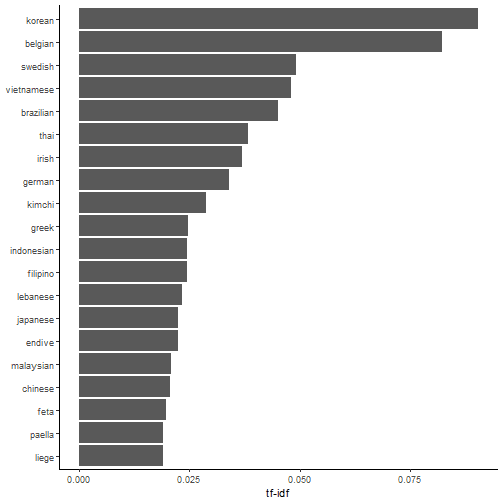
Now we can do a little visualisation of the top TF-IDF scores obtained

plot_geog <- geog_words %>%
  arrange(desc(tf_idf)) %>%
  mutate(word = factor(word, levels = rev(unique(word))))

plot_geog %>%
  top_n(20) %>%
  ggplot(aes(word, tf_idf)) +
  geom_col() +
  labs(x = NULL, y = "tf-idf") +
  coord_flip() +
  theme_classic()

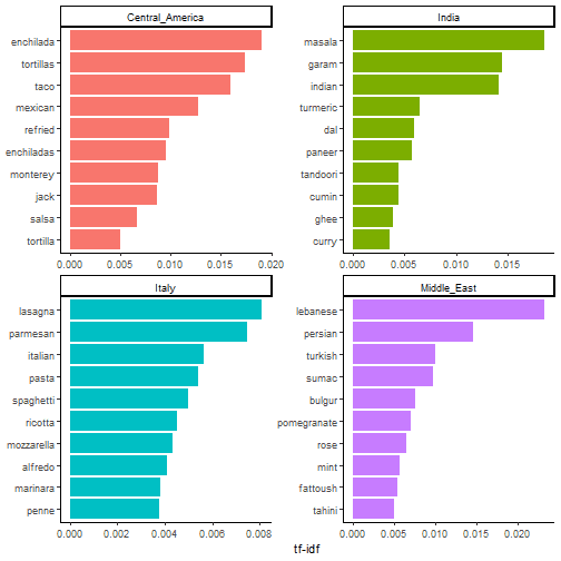
Country names dominate the top of the charts while other cuisine specific ingredients (e.g. Kimchi) also rank highly. A plot of the top 10 TF-IDF scores for selected regions also seem to produce sensible results.

plot_geog %>%
  filter(geog=="Italy" | geog=="India" |
         geog=="Central_America" | geog=="Middle_East") %>%
  group_by(geog) %>%
  arrange(geog, desc(tf_idf)) %>%
  top_n(10) %>%
  ungroup %>%
  ggplot(aes(word, tf_idf, fill = geog)) +
  geom_col(show.legend = FALSE) +
  labs(x = NULL, y = "tf-idf") +
  facet_wrap(~geog, ncol = 2, scales = "free") +
  coord_flip() +
  theme_classic()

Top 10 TF-IDF scores for selected regions

Subsequently, I match the TF-IDF scores for each word to the product description given by the Nielsen dataset. The scores are then normalised such that they sum up to one. This gives the metric a probabilistic interpretation, where the weight for a particular product can be thought of as the naive bayes estimate.^[Interestingly, while the TF-IDF approach seems relatively intuitive and sensible, the theoretical groundings for it are far less established. Nonetheless, it has be shown to be far better than traditional naive bayes for text categorisation purposes. See Kibriya et.al. (2004) for a comparison. ]

Using the dataset of household purchases, I am then able to calculate each household geographical region weighted expenditure share, which is the dependent variable in my regression analysis.

Other updates

On top of working on the actual regression analysis, I have also started collecting a 2nd set of food-region terms. Using two different data sources where the errors are quite likely uncorrelated would give me a better signal of the dependent variable, reducing problems of measurement error.

The next update should be quite a big one and would bring all the previous blog posts together so stay tune (if you are following).