Examining the Changes in Religious Beliefs - Part 2

In a previous post, I took a look at the distribution of religious beliefs in Singapore. Having compiled additional characteristics across 3 time periods (2000, 2010, 2015), I decided to write a follow-up post to examine the changes across time.

The dataset that I will be using is aggregated from the 2000 and 2010 Census as well as the 2015 General Household Survey. It covers most of the interesting social-economic variables with geographical variation that is released on Singstat's Table Builder. I compiled the various csv files and transform it into a format that can be easily used for analysis. The full dataset and cleaning files can be downloaded from my Github folder should you wish to have a go at it. The shapefiles used for mapping can be downloaded from https://data.gov.sg/. I used Master Plan 1998, 2008 and 2014 planning area boundaries which correspond to the geographical divisions used for the 3 surveys.

The following edits were made to the raw tables before appending them together:

• Consistent variable names and data entry fields were used where possible

• All values are in exact numbers instead of some being stated in thousands

• Only the main regions are extracted

• Data was transformed into a long format

Analysis

First, some preliminary data prep. I omit most of the steps to check for consistency across shapefiles covered in the previous post.

sg_plan_2015 <- readOGR(dsn=GIS_path, layer="MP14_PLNG_AREA_WEB_PL", verbose=FALSE)
sg_plan_2010 <- readOGR(dsn=GIS_path, layer="MP08_PLNG_AREA_NO_SEA_PL", verbose=FALSE)
sg_plan_2000 <- readOGR(dsn=GIS_path, layer="MP98_PLNG_AREA_NO_SEA_PL", verbose=FALSE)
df <- readRDS(data_path)

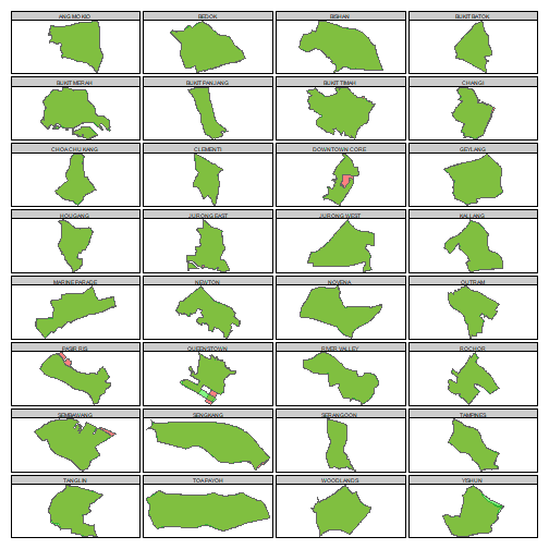
Before we start analysing the trends across time, one should ask how comparable the planning boundaries are across the years. To do so, we identify common regions across the master plans and do a plot to compare the difference in shape across the years.¹

region2000 <- unique(df[df$Year==2000,]$Level_3)
region2010 <- unique(df[df$Year==2010,]$Level_3)
region2015 <- unique(df[df$Year==2015,]$Level_3)
common_region <- region2010[region2010 %in% region2000]
common_region <- common_region[common_region %in% region2015]
sg_plan_2015c <- sg_plan_2015[sg_plan_2015$PLN_AREA_N %in% toupper(common_region),]
sg_plan_2000c <- sg_plan_2000[sg_plan_2000$PLN_AREA_N %in% toupper(common_region),]

tm_shape(sg_plan_2015c) +
  tm_polygons(col="red", alpha=0.5) +
  tm_facets("PLN_AREA_N", free.coords=TRUE) +
tm_shape(sg_plan_2000c) +
  tm_polygons(col="green", alpha=0.5) +
  tm_facets("PLN_AREA_N", free.coords=TRUE)

The light green regions are areas present in the 2000 Master Plan but not in the 2015 Master Plan while the opposite holds for the red regions. The dark green regions show the intersection of the two plans. It appears that most of the planning regions are very similar across 15 year period (unlike electoral boundaries). This justifies the comparison of values across the surveys.

Next, let us take a look at the variables present in the dataset:

names(df)

## [1] "Year"    "survey"  "content" "Level_1" "Level_2" "Level_3" "Value"

unique(df$content)

## [1] "resident_hh_dwelling"    "resident_hh_income"
## [3] "resident_pop_GMI"        "resident_pop_industry"
## [5] "resident_pop_occupation" "resident_pop_religion"
## [7] "resident_pop_age"        "resident_pop_ethnic_sex"
## [9] "resident_pop_dwelling"

Level_1 corresponds to the main category that is used used to partition the dataset. Level_2 refers to the secondary variable that the values are sub-divided over. Only the "resident_pop_ethnic_sex" and "resident_pop_age" files contains addition data by sex.^[For the "resident_pop_age" file the division by age and sex is only available for 2015. For the other files, Level_2 = Total.] Value refer to the estimated number of people who belong into that particular category. To analyse a particular topic of interest, one can subset the rows that match the desired topic in the content column. Here's a small function that makes extraction easy. It also returns either the proportion of residents belonging to a particular category or the absolute value and creates addition columns calculating the difference between the values in 2015 and 2000.

#' This function extracts the required variables in wide form.
#' @param df dataframe containing the cleaned region data.
#' @param name name of content that is extracted
#' @param variable either "Value" or "prop"
#' @return data extract in wide form.
SelectData <- function(df, name, variable){

  data_total <- df%>%
    filter(content==name & Level_1=="Total" & Level_2=="Total") %>%
    rename(total = Value) %>%
    dplyr:: select(Year, Level_3, total)

  data <- df%>%
    filter(content==name & Level_1!="Total") %>%
    left_join(data_total, by=c("Year", "Level_3")) %>%
    mutate(prop = Value/total *100,
           Level_3 = toupper(Level_3))

  if(length(unique(data$Level_2))==1){
    data_wide <- data %>%
      dplyr::select_('Level_1', 'Level_3', variable, 'Year') %>%
      dcast(Level_3 ~ Level_1 + Year, value.var=variable)
    vec_names <- unique(data$Level_1)
    } else{
    data_wide <- data %>%
      dplyr::select_('Level_1', 'Level_2', 'Level_3', variable, 'Year') %>%
      dcast(Level_3 ~ Level_1 + Level_2 + Year, value.var=variable)
    vec_names <- as.vector(outer(unique(data$Level_1), unique(data$Level_2), paste, sep="_"))
    }

  tryCatch(
    for(i in 1:length(vec_names)){
      data_wide[,paste0(vec_names[i], "_diff")] <-
        data_wide[,paste0(vec_names[i], "_2015")] - data_wide[,paste0(vec_names[i], "_2000")]
    },
    error = function(e) print("Err: Not all columns have data in 2015 and 2000"))
  return(data_wide)

}

The if clause is used to deal with the need to handle contents with and without a secondary sub-division column (i.e. Level_2). As a follow up on the previous post examining the distribution of religious beliefs in Singapore, let us extract the religion related data and examine the changes across time. For consistency, I also create a composite Christianity group. As per the previous post, I visualise the changes on the current map of Singapore using the regions from the 2014 Master Plan.

religion_data <- SelectData(df, "resident_pop_religion", "prop")

for (i in c(2000,2010,2015)){
  religion_data[,paste0("Christianity_",i)] <-
    religion_data[,paste0("Christianity Catholic_",i)] +
    religion_data[,paste0("Christianity Other Christians_",i)]
}

religion_data$Christianity_diff <- religion_data$Christianity_2015 - religion_data$Christianity_2000

sg2 <- st_as_sf(sg)
religion_map <- left_join(sg2, religion_data, by = c("PLN_AREA_N" = "Level_3"))

Figure 1 shows the growth of Christianity and no religious beliefs. Both groups experienced the largest increase over the 15 year period.

tm_shape(religion_map) +
  tm_polygons(c("Christianity_diff", "No Religion_diff"), colorNA="light grey", title="Proportion (%)") +
  tm_facets(free.scales = FALSE, nrow=1) +
  tm_layout(panel.labels=c("Christianity","No Religion"))

To breakdown the growth Christianity, one can examine the growth of Catholicism vs other Christian beliefs. While both grew over this time frame, the biggest increase can be attributed to the growth of other Christian believers.

tm_shape(religion_map) +
  tm_polygons(c("Christianity Catholic_diff", "Christianity Other Christians_diff"), colorNA="light grey", title="Proportion (%)")+
  tm_facets(free.scales = FALSE, nrow=1) +
  tm_layout(panel.labels=c("Catholic","Other Christians"))

Figure 3 shows an interesting picture of the decline in Buddhism and Taoism. The fall in the number of self-professed Buddhist is really significant over the 15 year period. I think part of the decline may be due to greater awareness over the differences in Buddhism and Taoism, resulting in more people claiming to be Taoist rather than Buddhist in the 2015 survey. Yet, the overall picture points to a decline in such beliefs. It would be nice to have a breakdown of religious beliefs by age to explore this issue further...

tm_shape(religion_map) +
  tm_polygons(c("Buddhism_diff", "Taoism_diff"), colorNA="light grey", title="Proportion (%)")+
  tm_facets(free.scales = FALSE, nrow=1) +
  tm_layout(panel.labels=c("Buddhism","Taoism"))

The share of believers of Islam has also declined as a fraction of the total resident population while the fraction of the population who subscribes to Hinduism remained relatively stable over the past 15 years.

tm_shape(religion_map) +
  tm_polygons(c("Islam_diff", "Hinduism_diff"), colorNA="light grey", title="Proportion (%)")+
  tm_facets(free.scales = FALSE, nrow=1) +
  tm_layout(panel.labels=c("Islam","Hinduism"))

It would be really interesting to ask what factors led to the growth of Christianity or 'No Religious beliefs' over this time period. To what extent can a change in the proportion of races or demographic trends explain this trend? Ideally, one would like to have a panel of respondents and analyse the change in individual beliefs over time. It might seem impossible to make inference from survey results released at the aggregate level, or is it? In the subsequent post I plan to create a pseudo panel using publicly available data and further explore this issue. At the very least, we should get some interesting cross-sectional correlations.

Bonus

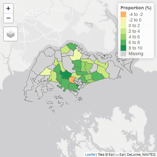
The tmap package also makes it very easy to produce interactive maps using the tmap_leaflet function.^[Note that the id variable assigned in the tm_polygons function only makes sense in the interactive view.] Here I reproduce the plot showing the growth of Christianity:

chr_map <- tm_shape(religion_map) +
  tm_polygons("Christianity_diff", colorNA="light grey", title="Proportion (%)",
  id="PLN_AREA_N")

tmap_leaflet(chr_map)